Duplicate data is expensive, distorts reports, and wastes marketing resources. Here are the steps for removing duplicates from Excel spreadsheets:
How to Remove Duplicates in Excel
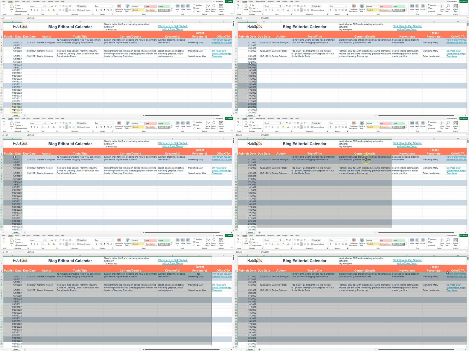
1. Select the cells you wish to remove duplicates from.
Click on a cell and hold down the left mouse button. Then drag the cursor over the other cells you want to select.
Or, use the Shift + arrow keyboard shortcut to select the range you want.
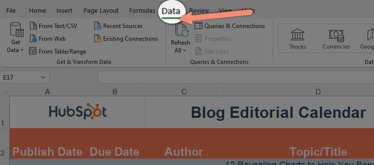
2. Click on the “Data” tab at the top.
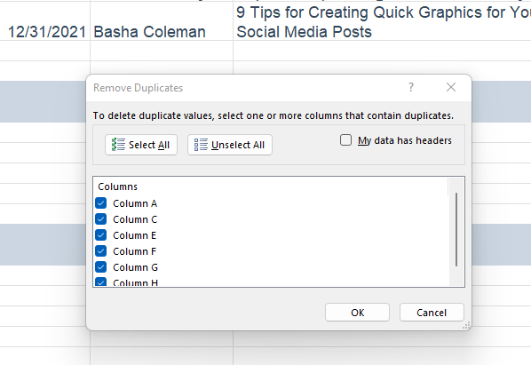
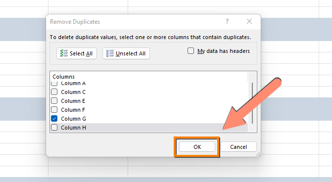
3. Click “Remove Duplicates” to reveal a pop-up.

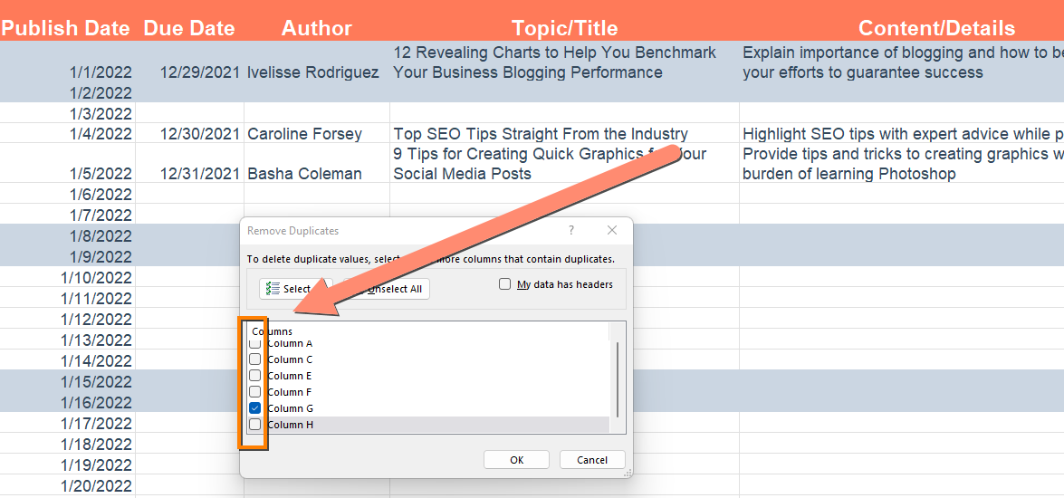
4. Uncheck any columns with data you want to keep.
5. Click OK to delete the duplicates.
Excel will keep the first occurrence of the value by default.
Also Read: How to Fix Long File Names in Windows 10?
How to Highlight Duplicates in Excel
Sometimes, you want to see the duplicate data before you delete it. Here’s how to find duplicate data in Excel:
1. Select the cells you wish to check for duplicates.
Click on a cell and hold down the left mouse button. Then drag the cursor over the other cells you want to select.
Or, use the Shift + arrow keyboard shortcut to select the range you want.
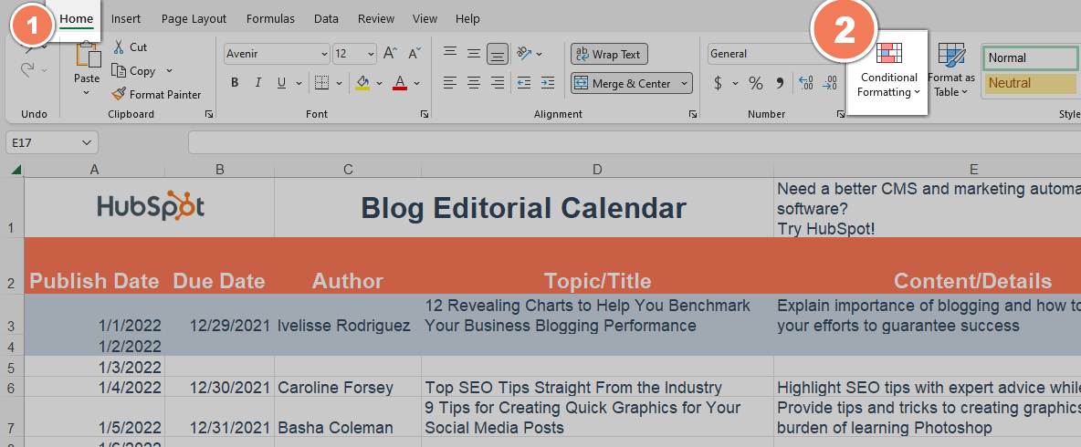
2. Click “Conditional Formatting” from the home tab to reveal a drop-down.
First, navigate to the home tab if you’re on a different tab.
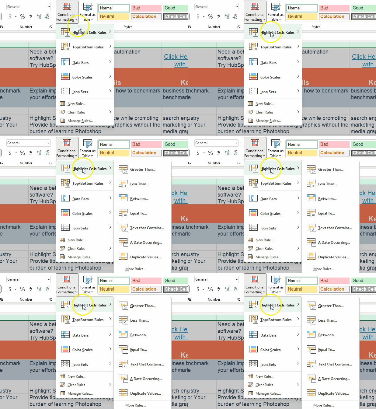
Click on “Conditional Formatting” to reveal a dropdown.
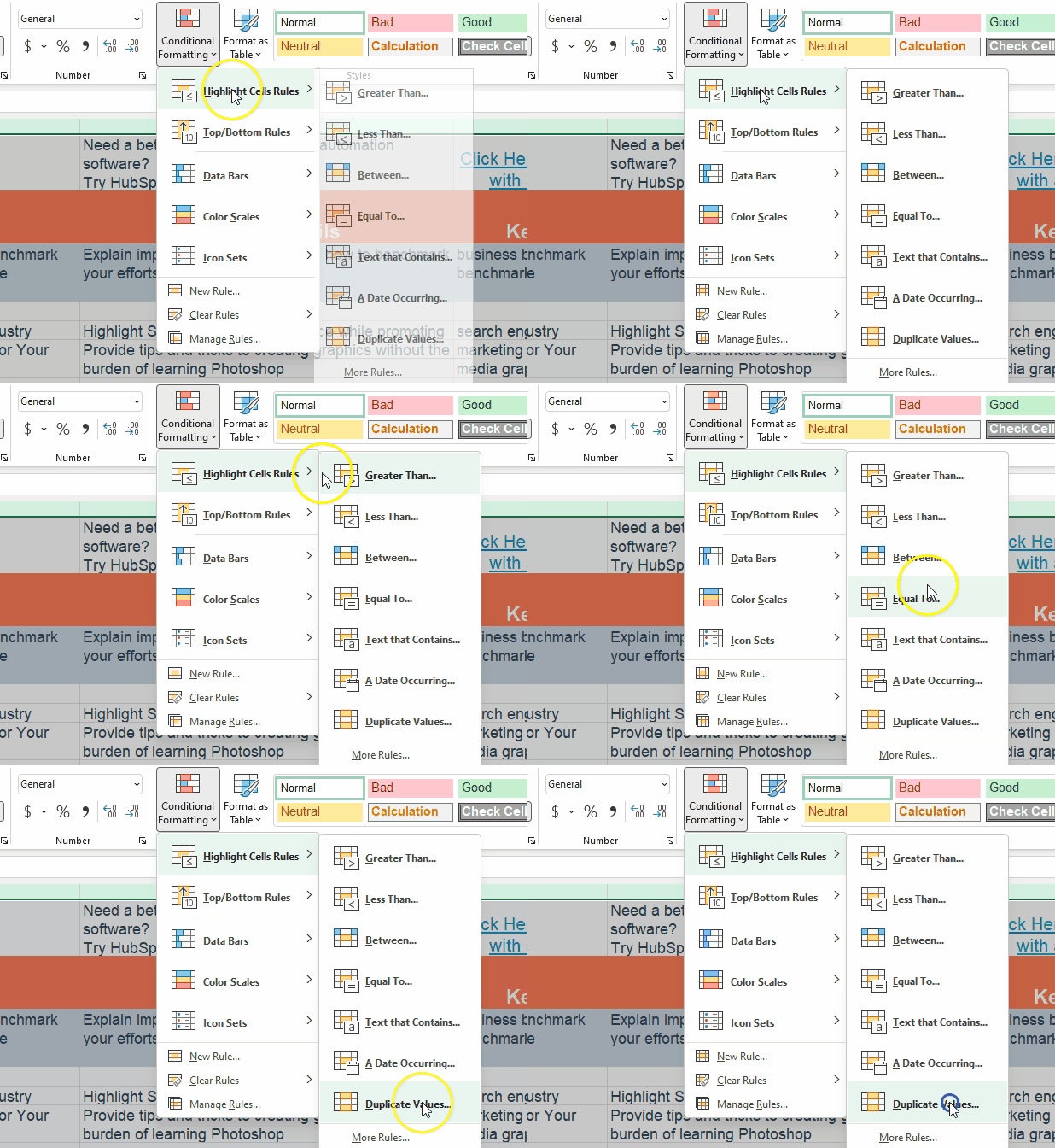
3. Hover over “Highlight Cell Rules”
4. Choose “Duplicate Values” from the options.
5. Pick the formatting option you want and click OK.
You’ll find all duplicates highlighted in the formatting style you choose.
Now you know how to find and remove duplicates in Excel!
Want more Excel automation hacks? Excel templates are a good place to start. They come pre-formatted with formulas that help you automate projections and more.

